Working with SAnTex#
In a Python working environment, import SAnTex’s modules and Python libraries:
from santex.ebsd import EBSD
from santex.tensor import Tensor
from santex.material import Material
from santex.isotropy import Isotropy
import pandas as pd
Load the EBSD file:
ebsdfile = EBSD("fdmrn02x01.ctf")
This loads the ebsd.ctf file in the Python object ebsdfile of class EBSD, from which users are able to call methods for further processing, cleaning of the ebsd data, and ultimately calculate elastic properties.
This loads the ebsd.ctf file in the python object ebsdfile of class EBSD, from which users are able to call methods for further processing, cleaning of the ebsd data, and ultimately calculate elastic properties.
Class: In Python, a class is a blueprint for creating objects. It defines the structure and behavior of objects of that type. Think of it as a template or a prototype that encapsulates data (attributes) and methods (functions) that operate on that data.
Object: An object, also known as an instance, is a unique entity that is created based on the structure defined by its class. When an object is instantiated, it inherits the attributes and methods defined in its class, but can also have its own unique state and behavior.
Note: The ebsd.ctf should be located in the directory this notebook is being run from. But you may provide a relative path like data/ebsd.ctf or an absolute import such as /Users/myname/Documents/ebsd/ebsd.ctf.
Available methods in the EBSD class#
To list the phases present in the ebsd file:
phases_available = ebsdfile.phases()
print(phases_available)
Load the ebsd file into a pandas dataframe df, via invoking the get_ebsd_data()
method from the EBSD class: Note: this dataframe df is critical as it holds
information of all the euler angles and the ebsd data.
df = ebsdfile.get_ebsd_data()
To look into the contents of the df, enter the following directive:
print(df)
To look into the data header of the EBSD file, following can be used:
ebsd_data_header = ebsdfile.get_ebsd_data_header()
print(ebsd_data_header)
To look at the index of phase, phases, and relative abundence, follwoing can be entered:
phases = ebsdfile.phases()
print(phases)
To get the euler angles of a certain phase, lets say phase = 1 in this case is Forsterite, enter the following:
forsteriteEulerAngles = ebsdfile.get_euler_angles(phase = 1, data = df)
print(forsteriteEulerAngles)
To plot this ebsd file, following can be enterred:
ebsdfile.plot(df)
This will plot the ebsd file in the default orientation of x2east and zOutOfPlane.
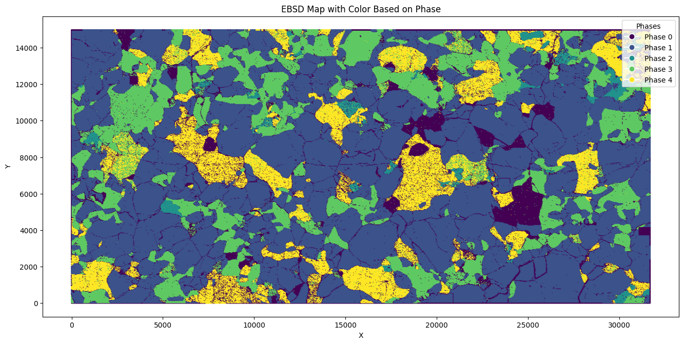
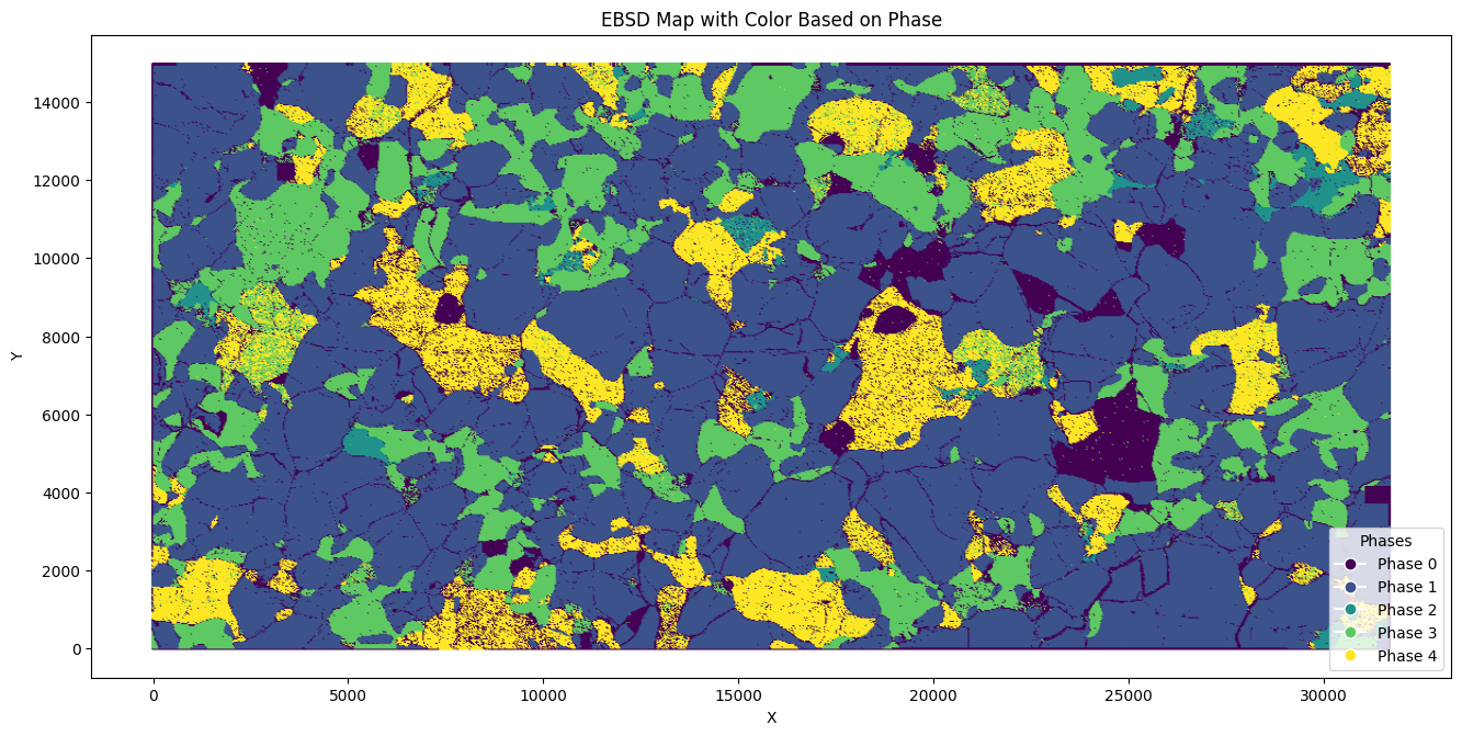
To save this image, following can be used:
ebsdfile.plot(df, cmap = "viridis", save_image= True, image_filename= "ebsd.jpg", legend_location="lower right")
Plotting Conventions#
Following are the keywords to orient sample reference plane and to store in a new dataframe, and plot it
1. sample_ref = ["x2east", "zOutOfPlane"]
2. sample_ref = ["x2west", "zOutOfPlane"]
3. sample_ref = ["x2north", "zOutOfPlane"]
4. sample_ref = ["x2south", "zOutOfPlane"]
5. sample_ref = ["x2east", "zIntoPlane"]
6. sample_ref = ["x2west", "zIntoPlane"]
7. sample_ref = ["x2north", "zIntoPlane"]
8. sample_ref = ["x2south", "zIntoPlane"]
To rotate the ebsd dataframe to x2east and zIntoPlane, do the following:
rotated_df = ebsdfile.plot_rotate_ebsd(sample_ref = ["x2east",
"zIntoPlane"], ebsd_df = df)
This rotates the ebsdfile in the specified convention, and saves the rotated dataframe in user-defined variable rotated_df
To plot this rotated_df, user can enter the following command:
rotated_df = ebsdfile.plot_rotate_ebsd(sample_ref = ["x2east",
"zIntoPlane"], ebsd_df = df)
Note: ebsdfile object created initaially from ebsdfile = EBSD('ebsd.ctf') can be reused for methods of EBSD object. For example, to plot the rotated dataframe, following can be entered:
ebsdfile.plot(rotated_df)

To rotate the EBSD data to match the SEM orientation in any custom angles, a user can enter the angles in Bunze ZXZ format as:
angles = (180, 0, 0)
updatedebsd = ebsdfile.rotate_ebsd(rotated_df, angles)
To view the current orientations, a user can always look at the ebsd plot using:
ebsdfile.plot(updatedebsd)

Get the phases names using the following:
phases_names = ebsdfile.phases_names()
print(phases_names)
Cleaning EBSD data#
In this example, to clean the EBSD dataset we successively remove grains with large mean angular deviation (MAD) of 0.8, reconstruct grains with grain boundaries misorientation ≥ 10 degrees, and remove grains smaller than 7 pixels.
Remove the phases which are mis-indexed (enter the endex of the phases):#
df = ebsdfile.filter_by_phase_number_list(df = updatedebsd, phase_list = [0, 2])
Remove pixel data with MAD higher than a user specified value#
To remove pixels with mean angular deviation e.g. (MAD) > 0.8, and store the cleaned dataset into a new dataframe called filtered_df:
filtered_df = ebsdfile.filter_MAD(df, 0.8)
Reconstruct grains with boundaries whose misorientation exceeds a minimum of 10 degrees:#
To reconstruct grains with misorientation ≥ 10 degrees and store the cleaner dataset into a new dataframe called df_grain_boundary:
phases_names = ebsdfile.phases_names()
phases_names = phases_names['phase'].tolist()
phases_names.insert(0, "na")

df_grain_boundary = ebsdfile.calc_grains(df = filtered_df, threshold = 10, phase_names=phases_names, downsampling_factor=10)
Note: Here the downsampling_factor is applied just for speedy handson!
Remove small grains#
User can remove grains smaller than e.g. 7 pixels, and store the cleaner dataset into a new dataframe called filtered_df_grain_boundary:
filtered_df_grain_boundary = ebsdfile.filter_by_grain_size(df_grain_boundary, phases_names, min_grain_size=7)
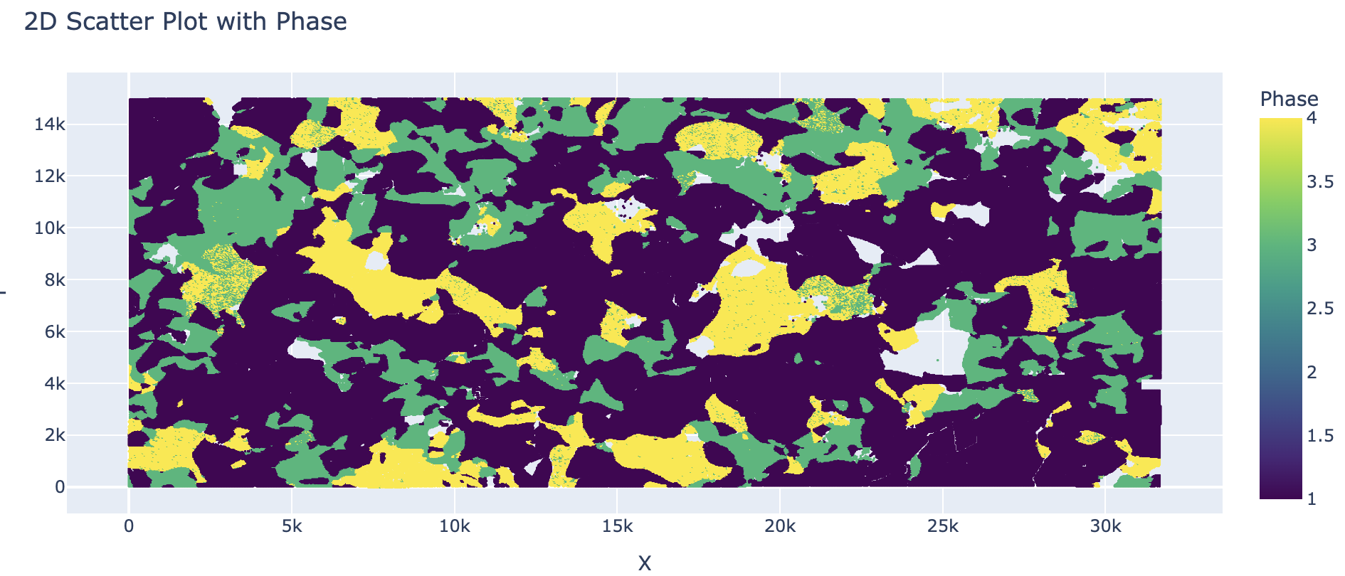
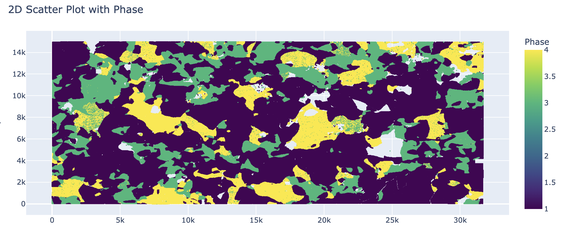
Compare original and clean datasets#
ebsdfile.plot()
ebsdfile.plot(data = filtered_df_grain_boundary)

The plot method of the EBSD class can take in a few parameters namely,
data (pandas.DataFrame, optional): DataFrame containing EBSD data. If not provided, uses stored data. rotation_angle (int, optional): Angle by which to rotate the EBSD data (in degrees). Accepts 0, 90, 180, 270. inside_plane (bool, optional): If True, rotates the EBSD data inside the plane. If False, rotates outside the plane. Default is True. mirror (bool, optional): If True, mirrors the EBSD data horizontally before rotating. Default is False. save_image (bool, optional): If True, saves the plot as an image. Default is False. image_filename (str, optional): Filename to use when saving the image. Required if save_image is True. dpi (int, optional): Dots per inch for the saved image. Default is 300. cmap (str, optional): Colormap to use for plotting. Default is ‘viridis’. legend_location (str, optional): Location of the legend. Options are ‘upper right’, ‘upper left’, ‘lower right’, ‘lower left’. Default is ‘upper right’.
Calculating Anisotropy from EBSD file#
To prepare the dataframe, the user can instanciate Material class as follows, be sure to check if the Material class is imported via from santex.material import Material:
material_instance = Material()
The densities are within the santex package registry, and can be accessed via the following directive. The pressure in GPa (here example: 2GPa) and Temperature (here 1500 degrees Celsius) can be entered as:
rho_Fo = material_instance.load_density("Forsterite", pressure = 2, temperature = 1500)
rho_diop = material_instance.load_density("Diopside", pressure = 2, temperature = 1500)
rho_ens = material_instance.load_density("Enstatite", pressure = 2, temperature = 1500)
The registry for elastic tensors within santex can be accessed via the following commands. The pressure and temperacture conditions can be entered via the keyword PRESSURE and TEMP
cij_Fo = material_instance.voigt_high_PT('Forsterite', PRESSURE = 2, TEMP = 1500)
cij_ens = material_instance.voigt_high_PT('Enstatite', PRESSURE = 2, TEMP = 1500)
cij_diop = material_instance.voigt_high_PT('Diopside', PRESSURE = 2, TEMP = 1500)
For preparing dataframes for seismic anisotropy, the elasticstiffness tensors and densities needs to be passed as a list, as:
cij = [cij_Fo, cij_ens, cij_diop]
density = [rho_Fo, rho_ens, rho_diop]
The euler angles for the phases should also be bundled in list as:
Note: Make sure to import Anisotropy class first using from santex.anisotropy import Anisotropy
forsterite = ebsdfile.get_euler_angles(phase = 1, data=filtered_df_grain_boundary)
enstatite = ebsdfile.get_euler_angles(phase = 2, data=filtered_df_grain_boundary)
diopside = ebsdfile.get_euler_angles(phase = 3, data=filtered_df_grain_boundary)
euler_angles = [forsterite, enstatite, diopside]
The anisotropy can then be calculated as following:
average_tensor, average_density = ebsdfile.get_anisotropy_for_ebsd(cij, euler_angles, density)
anis = Anisotropy(average_tensor*10**9, average_density)
To look at the plots for the seismic velocities, following command can be entered:
anis.plot()
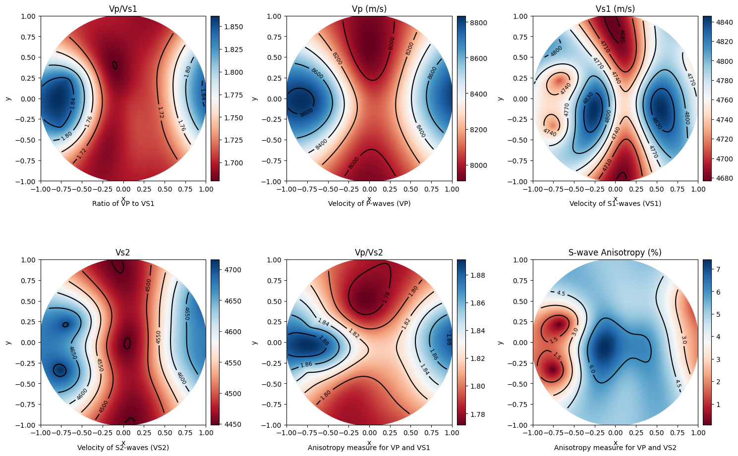
The plot() method can take in a few parameters namely:
- Parameters:
colormap (str): The colormap to use for plotting. Default is “RdBu_r”. step (int): The step size for theta and phi values. Default is 180. savefig (bool): Whether to save the plot as an image. Default is False. figname (str or None): The filename to save the plot. Required if savefig is True. dpi (int): The resolution of the saved image. Default is 300. save_format (str): svg or png or jpg
To look at the anisotropy values, maxvp, minvp, maxvs1, minvs1, etc.., folllowing command can be used:
anis.anisotropy_values()
This also returns a dictionary of values which can be used while modelling modal rocks with modal compositions at different pressure and temperacture.
This gives values such as:
Max Vp:  8449.545069720665
Min Vp:  7834.1684457727015
Max Vs1:  4843.772824149944
Min Vs1:  4577.275239228743
Max Vs2:  4661.180158160457
Min Vs2:  4555.315881762446
Max vs anisotropy percent:  6.110766862825683
Min vs anisotropy percent:  0.020842429078130564
P wave anisotropy percent:  7.558185340984474
S1 Wave anisotropy percent:  5.657493372889703
S2 Wave anisotropy percent:  2.297278183366879
Velocity difference:  287.209223367252
Vp/Vs1 ratio:  3.4012758430117644
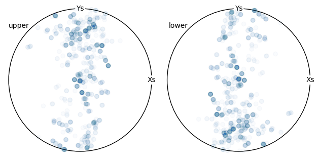
Pole Figures#
Pole figures are two dimensional representations of orientations. To illustrate this we define a random orientation with trigonal crystal symmetry
The pole figures can be calculated and plotted as:
ebsdfile.pf(df=filtered_df_grain_boundary,
    phase=1,
    crystal_symmetry='D2',
    random_val=True,
    uvw=[0, 1, 0],
    hemisphere='both',
    axes_labels=['Xs', 'Ys'],
    figure=None,
    show_hemisphere_label=None,
    grid=None,
    grid_resolution=None)
Following is the conversion tables which can be found from https://mtex-toolbox.github.io/HomepageOld/files/doc/symmetry_index.html . The crystal symmetry above should be defined as following convention. The user can enter the crystal symmetry as in either Schoenflies, or International, or Laue class, or Rotational axes convention.
id  crystal system  Schoen-  Inter-    Laue     Rotational
                    flies    national  class    axes
1   triclinic       C1       1         -1       1
2   triclinic       Ci       -1        -1       1
3   monoclinic      C2       211       2/m11    211
4   monoclinic      Cs       m11       2/m11    211
5   monoclinic      C2h      2/m11     2/m11    211
6   monoclinic      C2       121       12/m1    121
7   monoclinic      Cs       1m1       12/m1    121
8   monoclinic      C2h      12/m1     12/m1    121
9   monoclinic      C2       112       112/m    112
10  monoclinic      Cs       11m       112/m    112
11  monoclinic      C2h      112/m     112/m    112
12  orthorhombic    D2       222       mmm      222
13  orthorhombic    C2v      2mm       mmm      222
14  orthorhombic    C2v      m2m       mmm      222
15  orthorhombic    C2v      mm2       mmm      222
16  orthorhombic    D2h      mmm       mmm      222
17  trigonal        C3       3         -3       3
18  trigonal        C3i      -3        -3       3
19  trigonal        D3       321       -3m1     321
20  trigonal        C3v      3m1       -3m1     321
21  trigonal        D3d      -3m1      -3m1     321
22  trigonal        D3       312       -31m     312
23  trigonal        C3v      31m       -31m     312
24  trigonal        D3d      -31m      -31m     312
25  tetragonal      C4       4         4/m      4
26  tetragonal      S4       -4        4/m      4
27  tetragonal      C4h      4/m       4/m      4
28  tetragonal      D4       422       4/mmm    422
29  tetragonal      C4v      4mm       4/mmm    422
30  tetragonal      D2d      -42m      4/mmm    422
31  tetragonal      D2d      -4m2      4/mmm    422
32  tetragonal      D4h      4/mmm     4/mmm    422
33  hexagonal       C6       6         6/m      6
34  hexagonal       C3h      -6        6/m      6
35  hexagonal       C6h      6/m       6/m      6
36  hexagonal       D6       622       6/mmm    622
37  hexagonal       C6v      6mm       6/mmm    622
38  hexagonal       D3h      -62m      6/mmm    622
39  hexagonal       D3h      -6m2      6/mmm    622
40  hexagonal       D6h      6/mmm     6/mmm    622
41  cubic           T        23        m-3      23
42  cubic           Th       m-3       m-3      23
43  cubic           O        432       m-3m     432
44  cubic           Td       -43m      m-3m     432
45  cubic           Oh       m-3m      m-3m     432
46  icosahedral     I        532       -5-32/m  532
47  icosahedral     Ih       -5-32/m   -5-32/m  532
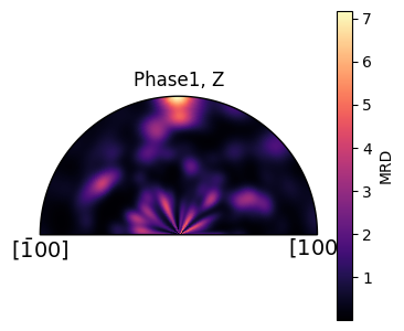
Inverse Pole Figure#
An inverse pole figure (IPF) is a way to represent the crystallographic orientation of a material relative to a fixed direction in the specimen. In simpler terms, it shows how the orientation of crystal planes aligns with a specific direction in the material, such as the direction of applied force or a particular axis in the specimen.
In order to illustrate the concept of inverse pole figures, let’s calculate the ipf and plot:
ebsdfile.ipf(df=filtered_df_grain_boundary,
    phase=1,
    vector_sample=[0, 0, 1],
    random_val=True,
    vector_title='Z',
    crystal_symmetry='D2',)
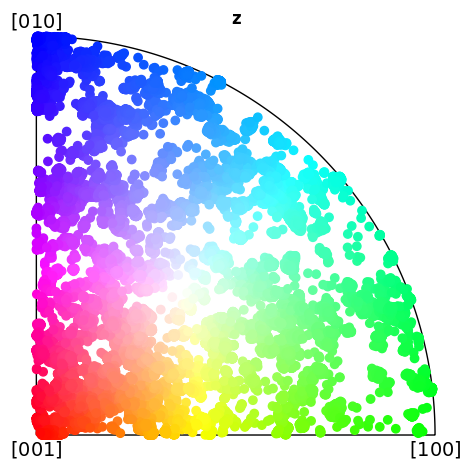
IPF color key#
ebsdfile.ipf_colorkey(df = df, phase=1, crystal_symmetry='D2')
Tensor analysis#
Stiffness tensors of phases are a 3*3*3*3 size, however, due to its symmetricity, it can also be written as a voigt notation of 6*6 matrix. A tensor can be rotated in Bunge Euler (ZXZ) convention
To initaially instanciate the Tensor Class, following needs to be inputted in python:
import numpy as np
from santex.tensor import Tensor

tensor = Tensor()
Let’s load some atiffness matrix values for forsterite written in voigt notation. The values can be seen in voigt matrix format
cij_forsterite = np.array([[320.5,  68.15,  71.6,     0,     0,     0],
[ 68.15,  196.5,  76.8,     0,     0,     0],
[  71.6,   76.8, 233.5,     0,     0,     0],
[   0,      0,      0,     64,     0,     0],
[   0,      0,      0,      0,    77,     0],
[   0,      0,      0,      0,     0,  78.7]])
To convert this voigt notation to tensor notation, a user can call voigt_to_tensor() method within Tensor class as follows:
cijkl_forsterite = tensor.voigt_to_tensor(cij_forsterite)
This gives a 3*3*3*3 array with the converted voigt in full tensor notation as seen
array([[[[320.5 ,   0.  ,   0.  ],
     [  0.  ,  68.15,   0.  ],
     [  0.  ,   0.  ,  71.6 ]],

    [[  0.  ,  78.7 ,   0.  ],
     [ 78.7 ,   0.  ,   0.  ],
     [  0.  ,   0.  ,   0.  ]],

    [[  0.  ,   0.  ,  77.  ],
     [  0.  ,   0.  ,   0.  ],
     [ 77.  ,   0.  ,   0.  ]]],


   [[[  0.  ,  78.7 ,   0.  ],
     [ 78.7 ,   0.  ,   0.  ],
     [  0.  ,   0.  ,   0.  ]],

    [[ 68.15,   0.  ,   0.  ],
     [  0.  , 196.5 ,   0.  ],
     [  0.  ,   0.  ,  76.8 ]],

    [[  0.  ,   0.  ,   0.  ],
     [  0.  ,   0.  ,  64.  ],
     [  0.  ,  64.  ,   0.  ]]],


   [[[  0.  ,   0.  ,  77.  ],
     [  0.  ,   0.  ,   0.  ],
     [ 77.  ,   0.  ,   0.  ]],

    [[  0.  ,   0.  ,   0.  ],
     [  0.  ,   0.  ,  64.  ],
     [  0.  ,  64.  ,   0.  ]],

    [[ 71.6 ,   0.  ,   0.  ],
     [  0.  ,  76.8 ,   0.  ],
     [  0.  ,   0.  , 233.5 ]]]])
The converted tensor can be converted back to voigt notation as:
Which then returns the 6*6 voigt notation of the tensor
array([[320.5 ,  68.15,  71.6 ,   0.  ,   0.  ,   0.  ],
   [ 68.15, 196.5 ,  76.8 ,   0.  ,   0.  ,   0.  ],
   [ 71.6 ,  76.8 , 233.5 ,   0.  ,   0.  ,   0.  ],
   [  0.  ,   0.  ,   0.  ,  64.  ,   0.  ,   0.  ],
   [  0.  ,   0.  ,   0.  ,   0.  ,  77.  ,   0.  ],
   [  0.  ,   0.  ,   0.  ,   0.  ,   0.  ,  78.7 ]])
Rotating tensors#
Rotating a Tensor in ZXZ Bunge Euler Convention#
To rotate a tensor using the ZXZ Bunge Euler convention, you perform a series of three rotations about specific axes. In this convention, the Euler angles \((\alpha, \beta, \gamma)\) represent rotations as follows:
Rotation by :math:`alpha` (first angle) around the Z-axis.
Rotation by :math:`beta` (second angle) around the X-axis.
Rotation by :math:`gamma` (third angle) around the Z-axis (again).
The full transformation matrix for the ZXZ convention is the product of three individual rotation matrices:
Rotation Matrices#
Rotation around the Z-axis by angle \(\theta\):
Rotation around the X-axis by angle \(\phi\):
Full Rotation Matrix#
The full rotation matrix for the ZXZ convention is:
Substitute the rotation matrices:
Rotating a Tensor#
Given a second-order tensor \(T\), after applying the rotation matrix \(R\), the rotated tensor \(T'\) can be obtained by:
where \(R^T\) is the transpose of the rotation matrix \(R\).
This process rotates the tensor according to the ZXZ Euler angles.
To rotate a tensor within santex, we can define alpha, beta and gamma in degrees, and then call the rotate_tensor() method within Tensor class as follows:
alpha = 10
beta = 20
gamma = 30

rotated_forsterite = tensor.rotate_tensor(cijkl_forsterite, alpha, beta, gamma)
voigt_rotated_forsterite = tensor.tensor_to_voigt(rotated_forsterite)
Now the same previous voigt tensor shown, is rotated, the new voigt notation of the rotated forsterite looks like:
array([[254.40669486,  83.60527452,  74.25170921,   2.25426383,
      9.1917399 ,  32.19107185],
   [ 83.60527452, 229.09177813,  77.9967799 ,   3.16662267,
      4.15506621,  24.85704921],
   [ 74.25170921,  77.9967799 , 228.39399978,  -5.76818554,
      4.58001959,  -1.68082112],
   [  2.25426383,   3.16662267,  -5.76818554,  72.58824371,
      7.02836206,   6.26816834],
   [  9.1917399 ,   4.15506621,   4.58001959,   7.02836206,
     73.39492984,   5.79247342],
   [ 32.19107185,  24.85704921,  -1.68082112,   6.26816834,
      5.79247342,  93.02059007]])
Material analysis#
The Material class from the Sage library is used for defining and working with materials calculations.
Material Module can be loaded as:
import numpy as np
from tabulate import tabulate
from santex.material import Material
The available material within the santex registry can be viewed as:
material_instance = Material()
phases_info = material_instance.available_phases()
print("Available Phases:")
print(phases_info)
This loads a list of materials present with their crystal systems and primary phase information as shown below:
Available Phases:
+---------------------------------------+---------------------+-----------------------------------+
|                 Phase                 |   Crystal System    |           Primary Phase           |
+---------------------------------------+---------------------+-----------------------------------+
|           Almandine-pyrope            |        Cubic        |              Garnet               |
|               Grossular               |        Cubic        |              Garnet               |
|               Majorite                |        Cubic        |              Garnet               |
|                Pyrope                 |        Cubic        |              Garnet               |
|              a_quartz_1               | Hexagonal/ Trigonal |              Quartz               |
|              a_quartz_2               | Hexagonal/ Trigonal |              Quartz               |
|              a_Quartz_3               | Hexagonal/ Trigonal |              Quartz               |
|              a_quartz_4               | Hexagonal/ Trigonal |              Quartz               |
|             a_quartz_696C             | Hexagonal/ Trigonal |              Quartz               |
|             a_quartz_700C             | Hexagonal/ Trigonal |              Quartz               |
|               Calcite_1               | Hexagonal/ Trigonal |              Calcite              |
|               Calcite_2               | Hexagonal/ Trigonal |              Calcite              |
|              Forsterite               |    Orthorhombic     |              Olivine              |
|               Fayalite                |    Orthorhombic     |              Olivine              |
|               Lawsonite               |    Orthorhombic     |              Olivine              |
|        Orthoenstatite (MgSiO3)        |    Orthorhombic     |              Olivine              |
|        Orthoenstatite (MgSiO3)        |    Orthorhombic     |              Olivine              |
|               Enstatite               |    Orthorhombic     |              Olivine              |
|       Bronzite (Mg0.8Fe0.2SiO3)       |    Orthorhombic     |              Olivine              |
|         Ferrosilite (FeSiO3)          |    Orthorhombic     |              Olivine              |
|                Biotite                |     Monoclinic      | Phyllosilicates and clay minerals |
|               Muscovite               |     Monoclinic      | Phyllosilicates and clay minerals |
|              Phlogopite               |     Monoclinic      | Phyllosilicates and clay minerals |
|            Illite-smectite            |     Monoclinic      | Phyllosilicates and clay minerals |
|                Dickite                |     Monoclinic      | Phyllosilicates and clay minerals |
|                Augite                 |     Monoclinic      |          Clinopyroxenes           |
|               Diopside                |     Monoclinic      |          Clinopyroxenes           |
|            Chrome-diopside            |     Monoclinic      |          Clinopyroxenes           |
|                Jadeite                |     Monoclinic      |          Clinopyroxenes           |
|               Omphacite               |     Monoclinic      |          Clinopyroxenes           |
|                Coesite                |     Monoclinic      |          Clinopyroxenes           |
|       Amphobole #1 Richterite1        |     Monoclinic      |             Amphibole             |
|       Amphobole #2 Kataphorite1       |     Monoclinic      |             Amphibole             |
|  Amphobole #3 Taramite-Tschermakite1  |     Monoclinic      |             Amphibole             |
| Amphobole #4 Hornblende-Tschermakite1 |     Monoclinic      |             Amphibole             |
|        Amphobole #5 Tremolite1        |     Monoclinic      |             Amphibole             |
|         Amphobole #6 Edenite1         |     Monoclinic      |             Amphibole             |
|         Amphobole #7 Edenite1         |     Monoclinic      |             Amphibole             |
|        Amphobole #8 Pargasite1        |     Monoclinic      |             Amphibole             |
|        Amphobole #9 Pargasite1        |     Monoclinic      |             Amphibole             |
|            Hornblende (#1)            |     Monoclinic      |             Amphibole             |
|            Hornblende (#2)            |     Monoclinic      |             Amphibole             |
|              Glaucophane              |     Monoclinic      |             Amphibole             |
|          Sanidine (Or83Ab15)          |     Monoclinic      |         Alkali feldspars          |
|          Sanidine (Or89Ab11)          |     Monoclinic      |         Alkali feldspars          |
|         Orthoclase (Or93Ab7)          |     Monoclinic      |         Alkali feldspars          |
|           Albite (Or0Ab100)           |      Triclinic      |       Plagioclase feldspar        |
|             An0 (Albite)              |      Triclinic      |       Plagioclase feldspar        |
|           An25 (Oligoclase)           |      Triclinic      |       Plagioclase feldspar        |
|            An37 (Andesine)            |      Triclinic      |       Plagioclase feldspar        |
|            An48 (Andesine)            |      Triclinic      |       Plagioclase feldspar        |
|          An60 (Labradorite)           |      Triclinic      |       Plagioclase feldspar        |
|          An67 (Labradorite)           |      Triclinic      |       Plagioclase feldspar        |
|           An78 (Bytownite)            |      Triclinic      |       Plagioclase feldspar        |
|           An96 (Anorthite)            |      Triclinic      |       Plagioclase feldspar        |
|               Kaolinite               |      Triclinic      |           Clay minerals           |
|                Nacrite                |      Triclinic      |           Clay minerals           |
+---------------------------------------+---------------------+-----------------------------------+
To look at any material properties, for example Diopside, get_properties_by_phase() can be called from Material class as follows:
material_instance = Material()

# Get properties for 'Diopside'
diopside_properties = material_instance.get_properties_by_phase('Diopside')
print("Material Properties for Diopside:")
print(tabulate(diopside_properties.items(), headers=["Property", "Value"], tablefmt="fancy_grid"))
print("\n")
which returns a formatted table of the properties of material (Diopside) as:
..code-block:: bash
Material Properties for Diopside: ╒═════════════════════════╤══════════════════════════╕ │ Property │ Value │ ╞═════════════════════════╪══════════════════════════╡ │ Crystal System │ Monoclinic │ ├─────────────────────────┼──────────────────────────┤ │ Primary Phase │ Clinopyroxenes │ ├─────────────────────────┼──────────────────────────┤ │ Phase │ Diopside │ ├─────────────────────────┼──────────────────────────┤ │ Density(g/cm3) │ 3.327 │ ├─────────────────────────┼──────────────────────────┤ │ C11 │ 237.8 │ ├─────────────────────────┼──────────────────────────┤ │ C22 │ 183.6 │ ├─────────────────────────┼──────────────────────────┤ │ C33 │ 229.5 │ ├─────────────────────────┼──────────────────────────┤ │ C44 │ 76.5 │ ├─────────────────────────┼──────────────────────────┤ │ C55 │ 73.0 │ ├─────────────────────────┼──────────────────────────┤ │ C66 │ 81.6 │ ├─────────────────────────┼──────────────────────────┤ │ C12 │ 83.5 │ ├─────────────────────────┼──────────────────────────┤ │ C13 │ 80.0 │ ├─────────────────────────┼──────────────────────────┤ │ C23 │ 59.9 │ ├─────────────────────────┼──────────────────────────┤ │ C15 │ 9.0 │ ├─────────────────────────┼──────────────────────────┤ │ C25 │ 9.5 │ ├─────────────────────────┼──────────────────────────┤ │ C35 │ 48.1 │ ├─────────────────────────┼──────────────────────────┤ │ C46 │ 8.4 │ ├─────────────────────────┼──────────────────────────┤ │ C14 │ 0 │ ├─────────────────────────┼──────────────────────────┤ │ C16 │ 0 │ ├─────────────────────────┼──────────────────────────┤ │ C24 │ 0 │ ├─────────────────────────┼──────────────────────────┤ │ C26 │ 0 │ ├─────────────────────────┼──────────────────────────┤ │ C34 │ 0 │ ├─────────────────────────┼──────────────────────────┤ │ C36 │ 0 │ ├─────────────────────────┼──────────────────────────┤ │ C45 │ 0 │ ├─────────────────────────┼──────────────────────────┤ │ C56 │ 0 │ ├─────────────────────────┼──────────────────────────┤ │ Crystal Reference Frame │ X||a* Y|| b Z||c │ ├─────────────────────────┼──────────────────────────┤ │ Study │ Collins and Brown [1998] │ ╘═════════════════════════╧══════════════════════════╛
To get the voigt matrix of Diopside to work with, get_voigt_matrix() of can be called as:
non_isotropic_phase = 'Diopside'
non_isotropic_voigt_matrix = material_instance.get_voigt_matrix(non_isotropic_phase)
print(f'Voigt matrix for {non_isotropic_phase}:')
print(tabulate(non_isotropic_voigt_matrix, tablefmt="pretty"))
which returns the voigt matrix for Diopside as:
Voigt matrix for Diopside:
+-------+-------+-------+------+------+------+
| 237.8 | 83.5  | 80.0  | 0.0  | 9.0  | 0.0  |
| 83.5  | 183.6 | 59.9  | 0.0  | 9.5  | 0.0  |
| 80.0  | 59.9  | 229.5 | 0.0  | 48.1 | 0.0  |
|  0.0  |  0.0  |  0.0  | 76.5 | 0.0  | 8.4  |
|  9.0  |  9.5  | 48.1  | 0.0  | 73.0 | 0.0  |
|  0.0  |  0.0  |  0.0  | 8.4  | 0.0  | 81.6 |
+-------+-------+-------+------+------+------+
For getting the voigt matrix at any given pressure and temperature for a material, voigthighPT() method can be called as:
cij_diopside = material_instance.voigt_high_PT('Diopside', PRESSURE = 2, TEMP = 1500)
This returns voigt matrix as this
array([[225.77,  83.47,  80.39,   0.  ,   8.25,   0.  ],
   [ 83.47, 175.8 ,  60.2 ,   0.  ,  10.07,   0.  ],
   [ 80.39,  60.2 , 219.36,   0.  ,  55.12,   0.  ],
   [  0.  ,   0.  ,   0.  ,  71.1 ,   0.  ,  12.93],
   [  8.25,  10.07,  55.12,   0.  ,  66.22,   0.  ],
   [  0.  ,   0.  ,   0.  ,  12.93,   0.  ,  74.76]])
To load the density at the different pressure and temperature, load_density() method can be called and pressure and temperature at 2GPa and 1500C can be parsed as:
rho_diopside = material_instance.load_density("Diopside", 2, 1500)
The above matrix which we get after evaluating at high temperature and pressure can be rotated given any 3 bunge euler rotations as:
from santex.tensor import Tensor
tensor = Tensor()
alpha = 10
beta = 20
gamma = 30

cijkl_diopside = tensor.voigt_to_tensor(cij_diopside)
rotated_forsterite = tensor.rotate_tensor(cijkl_diopside, alpha, beta, gamma)
cij_diopside_highpt = tensor.tensor_to_voigt(cijkl_diopside)
Hooke’s Law#
Hooke’s Law describes the behavior of certain materials when subjected to a stretching or compressing force. Hooke’s law can be expressed in terms of the elastic stiffness tensor and the strain tensor, as:
where \(\sigma_{ij}\) and \(\epsilon_{kl}\) are the components of the stress and strain tensors, respectively, while \(C_{ijkl}\) are the components of the elastic stiffness tensor. In this form, Hooke’s law is more general and can account for the anisotropy and directionality of the material’s elastic properties.
The pressure and temperature dependence of elastic constants is mainly linear but can include non-linear effects that can be approximated up to second-order terms using a Taylor series expansion, as outlined below:
In the current version of SAnTex, melt is considered as an isotropic phase with homogenous distribution within an anisotropic host rock, e.g., [@lee_modeling_2017:2017].
The fraction of melt, \(f\), can be controlled by the user. \(C_{\text{melt}}\) is the stiffness tensor of the melt. The approach currently incorporated in SAnTex overlooks the complex behavior of melt, including its viscosity, flow dynamics, and interaction with neighboring minerals, which can influence the overall anisotropic properties of the system. Future developments of SAnTex will aim to include more functionalities towards the calculation of melt-induced anisotropy.
Modal Mineral Composition of a rock and anisotropy#
within Santex, a user can parse a modal mineral composition for a rock and calculate its anisotropy as follows:
from santex.material import Material
from santex.anisotropy import Anisotropy

material = Material()
rock = ["Forsterite", "Diopside", "Enstatite"]
fraction = [0.6, 0.25, 0.15]
average_tensor, average_density = material.modal_rock(rock, fraction, 2, 1000)
anisotropy = Anisotropy(average_tensor*10**9, average_density)
values = anisotropy.anisotropy_values()
This returns a dictionary containing the anisotropy percent containing maxvp, minvp, minvs1, minvs2, maxvs1, maxvs2, max_vs_anisotropy_percent, min_vs_anisotropy_percent, p_wave_anisotropy_percent,
s1_wave_anisotropy_percent, s2_wave_anisotropy_percent, maxdvs, and AVpVs1
To plot the seismic velocities:
anisotropy.plot()
Isotropic Velocities analysis#
Isotropy module can be loaded as follows:
from santex.isotropy import Isotropy
isotropy = Isotropy()
To check the available phases, a user can invoke get_available_phases() within the Isotropy class as
isotropy.get_available_phases()
This gives a list of phases which are available in santex registry as is shown in below example
######################Available Phases######################
Material id: aqz       Material name: Alpha-Quartz
######################Available Phases######################
Material id: bqz       Material name: Beta-Quartz
######################Available Phases######################
Material id: coe       Material name: Coesite
######################Available Phases######################
Material id: hAb       Material name: High-T Albite
######################Available Phases######################
Material id: lAb       Material name: Low-T Albite
######################Available Phases######################
Material id: an       Material name: Anorthite
######################Available Phases######################
Material id: or       Material name: Orthoclase
######################Available Phases######################
Material id: san       Material name: Sanidine
######################Available Phases######################
Material id: alm       Material name: Almandine
######################Available Phases######################
Material id: gr       Material name: Grossular
######################Available Phases######################
Material id: py       Material name: Pyrope
######################Available Phases######################
Material id: fo       Material name: Forsterite
######################Available Phases######################
Material id: fa       Material name: Fayalite
######################Available Phases######################
Material id: en       Material name: Enstatite
######################Available Phases######################
Material id: fs       Material name: Ferrosillite
######################Available Phases######################
Material id: mgts       Material name: Mg-Tschermak
######################Available Phases######################
Material id: di       Material name: Diopside
######################Available Phases######################
Material id: hed       Material name: Hedenbergite
######################Available Phases######################
Material id: jd       Material name: Jadeite
######################Available Phases######################
Material id: ac       Material name: Acmite
######################Available Phases######################
Material id: cats       Material name: Ca-Tschermak
######################Available Phases######################
Material id: gl       Material name: Glaucophane
######################Available Phases######################
Material id: fgl       Material name: Ferroglaucophane
######################Available Phases######################
Material id: tr       Material name: Tremolite
######################Available Phases######################
Material id: fact       Material name: Ferroactinolite
######################Available Phases######################
Material id: ts       Material name: Tschermakite
######################Available Phases######################
Material id: parg       Material name: Pargasite
######################Available Phases######################
Material id: hb       Material name: Hornblende
######################Available Phases######################
Material id: anth       Material name: Anthophyllite
######################Available Phases######################
Material id: phl       Material name: Phlogopite
######################Available Phases######################
Material id: ann       Material name: Annite
######################Available Phases######################
Material id: mu       Material name: Muscovite
######################Available Phases######################
Material id: cel       Material name: Celadonite
######################Available Phases######################
Material id: ta       Material name: Talc
######################Available Phases######################
Material id: clin       Material name: Clinochlore
######################Available Phases######################
Material id: daph       Material name: Daphnite
######################Available Phases######################
Material id: atg       Material name: Antigorite
######################Available Phases######################
Material id: zo       Material name: Zoisite
######################Available Phases######################
Material id: cz       Material name: Clinozoisite
######################Available Phases######################
Material id: ep       Material name: Epidote
######################Available Phases######################
Material id: law       Material name: Lawsonite
######################Available Phases######################
Material id: pre       Material name: Prehnite
######################Available Phases######################
Material id: pump       Material name: Pumpellyte
######################Available Phases######################
Material id: lmt       Material name: Laumontite
######################Available Phases######################
Material id: wrk       Material name: Wairakite
######################Available Phases######################
Material id: br       Material name: Brucite
######################Available Phases######################
Material id: chum       Material name: Clinohumite
######################Available Phases######################
Material id: phA       Material name: Phase A
######################Available Phases######################
Material id: sill       Material name: Sillimanite
######################Available Phases######################
Material id: ky       Material name: Kyanite
######################Available Phases######################
Material id: sp       Material name: Mg-Spinel
######################Available Phases######################
Material id: herc       Material name: hercynite
######################Available Phases######################
Material id: mt       Material name: Magnetite
######################Available Phases######################
Material id: ilm       Material name: Ilmenite
######################Available Phases######################
Material id: rut       Material name: Rutile
######################Available Phases######################
Material id: ttn       Material name: Titanite
######################Available Phases######################
Material id: crd       Material name: Cordierite
######################Available Phases######################
Material id: scap       Material name: Scapolite
######################Available Phases######################
Material id: cc       Material name: Calcite
######################Available Phases######################
Material id: arag       Material name: Aragonite
######################Available Phases######################
Material id: mag       Material name: Magnesite
Following input parameters are inbuilt in ythe santex registry which initiates the isotropic properties calculation.
rho0: initial density
ao: coefficient of thermal expansion
akt0: isothermal bulk modulus, which is a measure of a material's resistance to compression under uniform pressure
dkdp: pressure derivative of the bulk modulus, indicating how the bulk modulus changes with pressure
amu0: shear modulus of the mineral. The shear modulus measures a material's resistance to deformation by shear stress
dmudp: pressure derivative of the shear modulus, indicating how the shear modulus changes with pressure
gam: gamma, first thermodynamic Gruinesen parameter
grun: second Gruneisen parameter, which is a measure of how a material's volume changes with temperature
delt: Debye temperature, which is a measure of the average vibrational energy of atoms in a solid.
User can call get_phase_constants() method as follows:
isotropy.get_phase_constants("Forsterite")
This returns a dictionary which looks like
    {'id': 'fo',
'name': 'Forsterite',
'rho0': 3222.0,
'ao': 6.13e-05,
'akt0': 127300000000.0,
'dkdp': 4.2,
'amu0': 81600000000.0,
'dmudp': 1.6,
'gam': 5.19,
'grun': 1.29,
'delt': 5.5}
We can get the following quantities at any given temperature and pressure for a material after calling the method calculate_seismic_properties()
density: density of material at any given pressure and temperature
aks: bulk modulus, The bulk modulus indicates how much a material will compress under pressure.
amu: Shear Modulus, The shear modulus is essential for understanding a material’s response to shear stress
vp: P-wave velocity at any given pressure and temperature
vs: swave velocity at any given pressure and temperature
vbulk: Bulk velocity.
akt: Isothermal bulk modulus, Similar to the bulk modulus, but specifically refers to the resistance to compression under constant 8. temperature conditions
The statement can be used as:
density, aks, amu, vp, vs, vbulk, akt = isotropy.calculate_seismic_properties('Forsterite', temperature=2000, pressure=2, return_vp_vs_vbulk=True, return_aktout=True)
which returns density, bulk modulus, shear modulus, vp, vs, bulk velocity and the isothermal bulk modulus at the specified pressure and temperature.
Hashin Shtrikman bounds for a modal rock#
Let’s define a rock with 62% Forsterite, 22% Diopside, and 16% enstatite (from the above ebsd data) as:
phases = ['fo', 'di', 'en']
fraction = [0.62, 0.22, 0.16]
Set modal composition as
ph, fr = isotropy.set_modal_composition(phase_list=phases, fraction_list=fraction)
Calculate the Hashin Shtrikman bounds for the rock as:
mid, upper, lower, rho = isotropy.hashin_shtrikman_bounds(phase_constant_list=ph, fraction_list=fr, temperature=1100, pressure=1.4, density_mix_calc=True)
3-D visualisation of vp, vs1, vs2 and vs splitting#
Firstly we have to calculate the anisotropy for a material as shown:
from santex.anisotropy import Anisotropy
from santex.material import Material

cij_diopside = material_instance.voigt_high_PT('Diopside', PRESSURE = 2, TEMP = 1500)
rho_diopside = material_instance.load_density('Diopside', 2, 1500)
anisotropy_instance = Anisotropy(cij_diopside, rho_diopside)
3-D visualtisation of vp can be done as
anisotropy_instance.plotter_vp(rho_diopside, cij_diopside)
For vs1:
anisotropy_instance.plotter_vs1(rho_diopside, cij_diopside)
For vs2:
anisotropy_instance.plotter_vs1(rho_diopside, cij_diopside)
For vs splitting:
anisotropy_instance.plotter_vs_splitting(rho_diopside, cij_diopside)